Unlock Your Sound: Stability AI's Stable Audio 3 Revolutionizes Audio Generation

Unlock Your Sound: Stability AI's Stable Audio 3 Revolutionizes Audio Generation

Imagine creating studio-quality audio in seconds. That's now a reality. Stability AI's Stable Audio 3 has arrived, a family of latent diffusion models engineered to transform audio generation and editing. A technical research paper details its architecture, but what can it *really* do? Stable Audio 3 generates high-fidelity stereo audio at 44.1 kHz, handles variable-length outputs, performs inpainting-based editing, and boasts blazing-fast inference speeds. From a professional standpoint, this opens doors for rapid prototyping in game development and film scoring.

What Makes Stable Audio 3 a Game Changer for Audio?

Is Stable Audio 3 just another incremental update? Not even close. It's a meticulously designed family of models—small, medium, and large—built on latent diffusion. This technique learns to generate audio by intelligently removing noise from a compressed audio representation (a latent). Trained on vast datasets of (noisy latent, audio) pairs, the model learns the complex mapping from noise to coherent, high-quality sound. Think of it as teaching an AI to sculpt sound from static.

The differences between the models? Capacity and maximum generation length. Here’s the breakdown:

• small-music: 459M diffusion transformer parameters, up to 2 minutes of music.
• small-sfx: 459M diffusion transformer parameters, sound effects up to 2 minutes.
• medium: 1.4B diffusion transformer parameters, extending to 6 minutes and 20 seconds for both music and sound effects.
• large: The 2.7B diffusion transformer parameter powerhouse, matching the medium model's 6 minutes and 20 seconds limit.

Here's the thing: the open weights for the small and medium models are on Hugging Face, inviting developers and researchers to experiment. The large model? That's under an enterprise license. Why the split? That's a question for Stability AI. This matters because wider access to the smaller models can accelerate innovation in audio applications.

Diving into the Architecture: Two Core Components

What's under the hood that makes this possible? Stable Audio 3's architecture relies on two key components:

• A semantic-acoustic autoencoder, SAME.
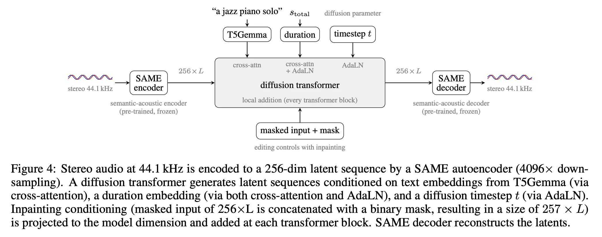
• A diffusion transformer, generating latent sequences conditioned on text prompts, duration specifications, and inpainting masks.

The SAME Autoencoder: Compressing Audio with Precision

SAME (Semantically-Aligned Music autoEncoder) converts stereo 44.1 kHz audio into a compact latent representation and reconstructs it. Its defining feature? A remarkable 4096× downsampling ratio, far exceeding the 1024× to 2048× ratios of previous audio autoencoders. This aggressive downsampling shrinks latent sequence lengths, enabling long-form audio generation even on standard hardware. Impressive, right? Industry analysis suggests this compression is key to making the model practical for widespread use.

That 4096× compression happens in two stages. First, a patching stage reshapes stereo audio into non-overlapping patches of 256 samples per channel (256× downsampling). Second, a Transformer Resampling Block (TRB) applies another 16× downsampling, using learnable output embeddings interleaved with the input sequence, all processed through a transformer. The result? A 256-dimensional latent sequence running at about 10.76 Hz for a 44.1 kHz input.

The SAME autoencoder trains using five loss types: spectral reconstruction, adversarial, diffusion alignment, semantic regression (predicting chroma and interaural level difference), and contrastive latent alignment. These ensure the latent preserves acoustic reconstruction quality and semantic structure. A soft-normalization bottleneck constrains the latent's scale, ensuring deterministic encoding. It's a complex dance of algorithms, all working in harmony.

Crucially, SAME remains frozen during diffusion training. The small models use SAME-S (108M parameters, optimized for CPU inference), while the medium and large models leverage SAME-L (852M parameters). Why freeze it? To maintain a stable base while the diffusion model learns.

The Diffusion Transformer: Generating Latent Sequences

The diffusion transformer works directly on the SAME latents. Conditioning happens through three key pathways:

1. Text: A frozen T5Gemma encoder generates a sequence of 256 embeddings, each 768-dimensional. Short prompts are padded to 256 using a learned embedding; longer prompts are truncated.
2. Duration: Encoded as a Fourier features vector and injected via Adaptive Layer Normalization (AdaLN) and cross-attention alongside the text prompt.
3. Inpainting: A binary mask, concatenated with the masked reference audio, is projected through a 2-layer MLP and added to the residual stream of each transformer block.

Each transformer block includes self-attention, cross-attention, local-additive conditioning for inpainting, and a SwiGLU feed-forward network. The medium and large models use differential attention, computing two separate attention maps using two (Q, K) pairs sharing one set of values V, then subtracting one map from the other to cancel out common attention patterns. Clever, huh? The transformer prepends 64 learnable memory embeddings before processing each sequence, providing a global context buffer that every position can attend to. These embeddings are removed before computing any loss.

Variable-Length Generation: A Breakthrough in Efficiency

Here's a big deal: Unlike many latent diffusion models that operate at a fixed maximum sequence length, Stable Audio 3 generates audio at variable lengths. This is achieved through three mechanisms:

• Variable-length flash attention and masked loss: Sequences shorter than the batch maximum are right-padded in latent space, and padding positions are excluded from self-attention and the loss calculation.
• Per-element timestep shifts: To compensate for the increased structure retention in longer sequences at a given noise level, the noise schedule shifts toward higher noise levels for longer sequences during training, using a logistic shift parameterized by µ.
• Silence augmentation: The signal region is randomly extended with pre-computed silence embeddings drawn from an exponential distribution, averaging 4 seconds. This teaches the model to terminate audio with natural silence.

The result? Inference cost scales directly with output duration. On an H200, the medium model generates 20 seconds of audio in about 0.62 seconds, while generating 380 seconds takes only 1.31 seconds. That said, real-world performance will vary.

The Three-Stage Training Pipeline: From Noise to Clarity

How did they train this beast? Stable Audio 3's training is divided into three stages:

Stage 1 — Flow Matching Pre-Training: The model learns a velocity field that transports Gaussian noise toward audio latents. Training uses minibatch optimal transport coupling via Sinkhorn iterations, pairing each data sample with the closest available noise vector in the batch. This streamlines training trajectories and minimizes crossing transport paths. Inpainting is integrated throughout, with one of three mask types sampled at each step: full mask, random segment masks, or a causal prefix mask for continuation.

Stage 2 — Distillation Warmup: A frozen copy of the flow matching model (the teacher) generates 15-step DPM++ trajectories with CFG scale 5. The student model is trained for 10,000 steps to directly map any intermediate noisy state to the teacher’s final denoised output in a single step, using an MSE loss. This collapses the multi-step ODE into a single-step denoiser. But the trade-off is that MSE regression tends to produce outputs that regress toward the conditional mean, potentially reducing fine-grained detail.

Stage 3 — Adversarial Post-Training: This stage replaces the MSE objective with a relativistic adversarial setup. A discriminator (initialized from the base flow matching model) evaluates the student’s one-step denoised outputs directly against real data. The teacher is discarded. The generator is trained with a relativistic adversarial loss (L_R) and a CLAP alignment loss (L_CLAP). The discriminator is trained with L_R and a contrastive loss (L_C) that penalizes it for ignoring text-audio alignment, training it to distinguish correctly paired audio-text pairs from shuffled ones. The adversarial setup allows the model to recover the perceptual sharpness lost during MSE distillation. While this holds for most audio types, some complex musical arrangements may still present challenges.